Title: Plot an equation containing two variables in C#

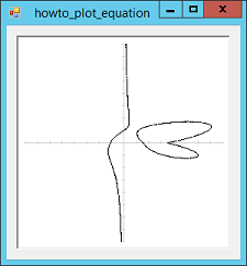
This example shows one way you can plot an equation containing two variables with the format F(x, y) = 0.

Some equations, such as y = 3 × x + 5, are easy to graph. Others are much harder. For example, how do you graph the following equation?

x³ / (|y| + 1) - 4 × x² + 4 × x × y² - y × 6 + 6 = 0

I don't know about you, but I wouldn't have guessed that this equation's graph looked like the picture shown above.

This program demonstrates one way to handle this problem.

First, if the equation is not already in the form F(x, y) = 0, convert it into that format. If the equation has non-zero pieces on each side of the equal sign, simply subtract one side to move it to the other. For example, the equation y = 3 × x + 5 is equivalent to y - (3 × x + 5) = 0.

Now the program loops over the area to plot. For each point in the area, it calculates the value of the function at that point and at the next point vertically and horizontally. If the sign of the values is different, then the function's value crossed from < 0 to > 0 or vice versa. In that case, the intermediate value theorem says the function must have taken the value 0 somewhere in that range (assuming the function is continuous) so the program plots the point.

The following code shows how the program loops over the area plotting points.

// Plot a function. private void PlotFunction(Graphics gr, float xmin, float ymin, float xmax, float ymax, float dx, float dy) { // Plot the function. using (Pen thin_pen = new Pen(Color.Black, 0)) { // Horizontal comparisons. for (float x = xmin; x <= xmax; x += dx) { float last_y = F1(x, ymin); for (float y = ymin + dy; y <= ymax; y += dy) { float next_y = F1(x, y); if ( ((last_y <= 0f) && (next_y >= 0f)) || ((last_y >= 0f) && (next_y <= 0f)) ) { // Plot this point. gr.DrawLine(thin_pen, x, y - dy, x, y); } last_y = next_y; } } // Horizontal comparisons. // Vertical comparisons. for (float y = ymin + dy; y <= ymax; y += dy) { float last_x = F1(xmin, y); for (float x = xmin + dx; x <= xmax; x += dx) { float next_x = F1(x, y); if ( ((last_x <= 0f) && (next_x >= 0f)) || ((last_x >= 0f) && (next_x <= 0f)) ) { // Plot this point. gr.DrawLine(thin_pen, x - dx, y, x, y); } last_x = next_x; } } // Vertical comparisons. } // using thin_pen. } // The function. // x^3 / (Abs(y) + 1) - 4 * x^2 + 4 * x * y^2 - y * 6 + 6 = 0 private float F1(float x, float y) { return (float)(x * x * x / (Math.Abs(y) + 1) - 4 * x * x + 4 * x * y * y - y * 6 + 6); }

You might be able to get a slightly better result by calculating the curve's partial derivatives, either analytically or by using Newton's method, but this method is a lot simpler.

Download the example to experiment with it and to see additional details.